PostGIS 2.1 on Caffeine: Raster, Topology, and pgRouting
Regina Obe and Leo Hsu
http://www.postgis.us http://www.bostongis.com
http://www.paragoncorporation.com http://www.postgresonline.com

Except where otherwise noted, content on these slides is licensed under a Creative Commons Attribution 4.0 International license.
Agenda
Beyond geometry and geography
Pixelated view of the world
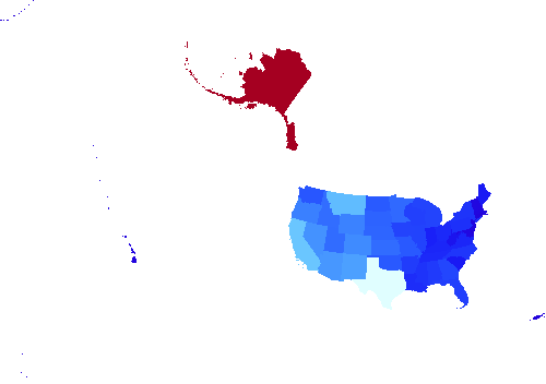
Relational view of the world
Costs along a network
Load OSM data
hstore needs to be installed before you can use --hstore-all or --hstore
Data from https://mapzen.com/metro-extracts (Chicago) chicago.osm.pbf
osm2pgsql -d presentation -H Y -U postgres -P 5438 -W \
-S default.style --hstore-all chicago.osm.pbfRaster
Rasters are matrixes that you can perform analysis on. They can also be rendered as pretty pictures. In PostGIS land, they live chopped into tiles in a table row in a column type called raster. They are often found dancing with geometries.
Let's see some rasters
We'll start with the serious (what real raster people work with) and move to the playful (what even your toddler can grasp).
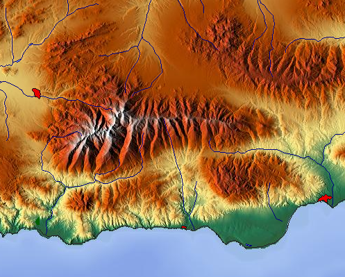
Digital Elevation Model (DEM)
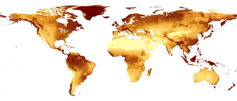
Climate
Temperature, water fall, climate change
Rasterization of a Geometry
Geometries can be rasterized
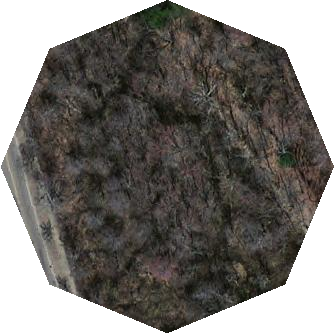
An aerial clip
Mona Lisa

Next we'll look at raster under a microscope
PostGIS raster under a microscope
- Tiles
- Pixels
- Bands
- Pixel Values
Rasters
Rasters are stored in table rows in a column of data type raster.

CREATE TABLE elevated(rid serial primary key, rast raster);
Tiles and Coverages
Rasters (especially those covering a large expanse of land) can be big so we chop them into smaller bits called tiles for easier analysis.
Tiles covering continguous non-overlapping areas of space with same kind of information we call:
A COVERAGE
Pixels as cells
Tiles are further broken down into pixels (or cells), organized into a matrix.
| Columns X | |
Rows Y | 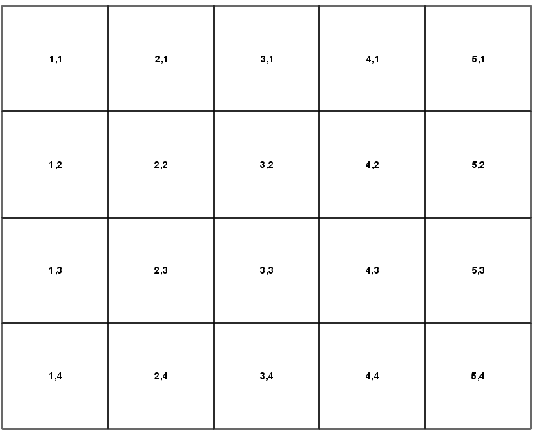 |
Numbering starts at the upper-left corner
Pixels: Geospatial Space
Example of pixel min spots in WGS lon lat
| Longitude | |
Latitude | 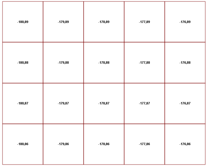 |
Note how Y coordinates are generally in reverse order of Pixel row numbering.
Raster is broken into 1 or more bands
Think of each band as a separate matrix storing a particular theme of data and particular numeric range.
One band can store elevation
Another temperature
Another vegetation
Another number of pizza restaurants in each area
If you just care about pretty pictures you can have a 4-band raster representing RGBA channels (bands) in your picture
Pixel Band Types
Bands are classified by the range of numeric data they can store and each band in a given raster can store a different range type of data.
- 1BB: 1-bit boolean
Bit Unsigned Integers (BUI): 2BUI, 4BUI, 8BUI, 16BUI, 32BUI
Bit Signed Integers (SI): 8BSI, 16BSI, 32BSI
Bit Floats (BF) - 32BF, 64BF
Pixel Values
Each pixel has slots for number of bands
3-banded raster means 3 values per pixel
Get data
- Pictures from http://en.wikipedia.org/wiki/Chicago
- Elevation data from http://www.webgis.com/terr_pages/IL/dem75/cook.html
Raster toolkit
GDAL: http://www.gdal.org
PostGIS raster is built on Gdal and wraps a lot of the functions of GDAL in an SQL wrapper
Commonly used command-line of GDAL
- gdalinfo: inspect a given raster
- gdal_translate: convert raster from one format to another
- gdalwarp: transform raster from one spatial projection to another and also changes format
Loading Data
raster2pgsql
raster2pgsql is a command-line tool packaged with PostGIS 2+ that allows loading data from various raster formats into PostGIS raster format. It generates a sql load file or you can pipe directly to PostgreSQL with psql.
raster2pgsql options
RELEASE: 2.2.0dev GDAL_VERSION=111 (r12973)
USAGE: raster2pgsql [<options>] <raster>[ <raster>[ ...]] [[<schema>.]<table>]
  Multiple rasters can also be specified using wildcards (*,?).

OPTIONS:
  -s <srid> Set the SRID field. Defaults to 0. If SRID not
     provided or is 0, raster's metadata will be checked to
     determine an appropriate SRID.
  -b <band> Index (1-based) of band to extract from raster. For more
      than one band index, separate with comma (,). Ranges can be
      defined by separating with dash (-). If unspecified, all bands
      of raster will be extracted.
  -t <tile size> Cut raster into tiles to be inserted one per
      table row. <tile size> is expressed as WIDTHxHEIGHT.
      <tile size> can also be "auto" to allow the loader to compute
      an appropriate tile size using the first raster and applied to
      all rasters.
  -P Pad right-most and bottom-most tiles to guarantee that all tiles
     have the same width and height.
  -R  Register the raster as an out-of-db (filesystem) raster. Provided
      raster should have absolute path to the file
 (-d|a|c|p) These are mutually exclusive options:
     -d  Drops the table, then recreates it and populates
         it with current raster data.
     -a  Appends raster into current table, must be
         exactly the same table schema.
     -c  Creates a new table and populates it, this is the
         default if you do not specify any options.
     -p  Prepare mode, only creates the table.
  -f <column> Specify the name of the raster column
  -F  Add a column with the filename of the raster.
  -n <column> Specify the name of the filename column. Implies -F.
  -l <overview factor> Create overview of the raster. For more than
      one factor, separate with comma(,). Overview table name follows
      the pattern o_<overview factor>_<table>. Created overview is
      stored in the database and is not affected by -R.
  -q  Wrap PostgreSQL identifiers in quotes.
  -I  Create a GIST spatial index on the raster column. The ANALYZE
      command will automatically be issued for the created index.
  -M  Run VACUUM ANALYZE on the table of the raster column. Most
      useful when appending raster to existing table with -a.
  -C  Set the standard set of constraints on the raster
      column after the rasters are loaded. Some constraints may fail
      if one or more rasters violate the constraint.
  -x  Disable setting the max extent constraint. Only applied if
      -C flag is also used.
  -r  Set the constraints (spatially unique and coverage tile) for
      regular blocking. Only applied if -C flag is also used.
  -T <tablespace> Specify the tablespace for the new table.
      Note that indices (including the primary key) will still use
      the default tablespace unless the -X flag is also used.
  -X <tablespace> Specify the tablespace for the table's new index.
      This applies to the primary key and the spatial index if
      the -I flag is used.
  -N <nodata> NODATA value to use on bands without a NODATA value.
  -k  Skip NODATA value checks for each raster band.
  -E <endian> Control endianness of generated binary output of
      raster. Use 0 for XDR and 1 for NDR (default). Only NDR
      is supported at this time.
  -V <version> Specify version of output WKB format. Default
      is 0. Only 0 is supported at this time.
  -e  Execute each statement individually, do not use a transaction.
  -Y  Use COPY statements instead of INSERT statements.
  -G  Print the supported GDAL raster formats.
  -?  Display this help screen.
Warm-up Exercise
What kind of rasters can we load?
raster2pgsql -GShould give you something like
Supported GDAL raster formats:
  Virtual Raster
  GeoTIFF
  National Imagery Transmission Format
  Raster Product Format TOC format
  ECRG TOC format
  Erdas Imagine Images (.img)
:
  Ground-based SAR Applications Testbed File Format (.gff
  ELAS
  Arc/Info Binary Grid
  Arc/Info ASCII Grid
  GRASS ASCII Grid
  SDTS Raster
  DTED Elevation Raster
  Portable Network Graphics
  JPEG JFIF
  In Memory Raster
:
  Graphics Interchange Format (.gif)
  Envisat Image Format
  Maptech BSB Nautical Charts
  X11 PixMap Format
  MS Windows Device Independent Bitmap
  SPOT DIMAP
  AirSAR Polarimetric Image
  RadarSat 2 XML Product
 :
Inspect metadata
Yes pictures have meta data, but don't care much about it as far as loading goes
gdalinfo Chicago_sunrise_1.jpgSize is 7550, 2400
Coordinate System is `'
Image Structure Metadata:
COMPRESSION=JPEG
INTERLEAVE=PIXEL
SOURCE_COLOR_SPACE=YCbCr
Corner Coordinates:
Upper Left ( 0.0, 0.0)
Lower Left ( 0.0, 2400.0)
Upper Right ( 7550.0, 0.0)
Lower Right ( 7550.0, 2400.0)
Center ( 3775.0, 1200.0)
Band 1 Block=7550x1 Type=Byte, ColorInterp=Red
Overviews: 3775x1200, 1888x600, 944x300
Image Structure Metadata:
COMPRESSION=JPEG
Band 2 Block=7550x1 Type=Byte, ColorInterp=Green
Overviews: 3775x1200, 1888x600, 944x300
Image Structure Metadata:
COMPRESSION=JPEG
Band 3 Block=7550x1 Type=Byte, ColorInterp=Blue
Overviews: 3775x1200, 1888x600, 944x300
Image Structure Metadata:
COMPRESSION=JPEG
Exercise: Load a folder of Pictures
In db
Don't waste your time with indexes and constraints. Don't bother tiling either
raster2pgsql -e -F -Y pics/*.jpg po.chicago_pics | psql -U postgres -d presentationExercise: Load a folder of Pictures
Keep out of database
For database snobs who feel rasters and gasp! pictures have no place in a database. Use the -R switch
Warning: path you register must be accessible by postgres daemon and for PostGIS 2.1.3+ , 2.0.6+ need to set POSTGIS_ENABLE_OUTDB_RASTERS environment variable. For 2.2+ have option of GUCs.
raster2pgsql -R -e -F -Y /fullpath/pics/*.jpg po.chicago_pics \
| psql -U postgres -d presentationGdalInfo: Inspect metadata before load
gdalinfo chicago-w.DEMSize is 1201, 1201 Coordinate System is: GEOGCS["NAD27", DATUM["North_American_Datum_1927", SPHEROID["Clarke 1866",6378206.4,294.978698213898 AUTHORITY["EPSG","7008"]], AUTHORITY["EPSG","6267"]], PRIMEM["Greenwich",0, AUTHORITY["EPSG","8901"]], UNIT["degree",0.0174532925199433, AUTHORITY["EPSG","9108"]], AUTHORITY["EPSG","4267"]] Origin = (-88.000416666666666,42.000416666666666) Pixel Size = (0.000833333333333,-0.000833333333333) Metadata: AREA_OR_POINT=Point Corner Coordinates: Upper Left ( -88.0004167, 42.0004167) Lower Left ( -88.0004167, 40.9995833) Upper Right ( -86.9995833, 42.0004167) Lower Right ( -86.9995833, 40.9995833) Center ( -87.5000000, 41.5000000) Band 1 Block=1201x1201 Type=Int16, ColorInterp=Undefined NoData Value=-32767 Unit Type: m
Exercise: Load Elevation data
Indexes are important, spatial ref is important, constraints are important too
And you want to tile cause it's gonna be a coverage where fast analysis of small areas is important.
raster2pgsql -I -C -e -F -Y -t auto -s 4267 dems/*.DEM po.chicago_dem \
| psql -U postgres -d presentationViewing and outputting rasters
Lots of options, but first a warning.
PostGIS 2.1.3+ and 2.0.6+, security locked down, so you'll need to set: POSTGIS_GDAL_ENABLED_DRIVERS to use built-in ST_AsPNG etc functions.
PostGIS 2.2+ allow to set using GUCS
Output with psql
Wrap your query in ST_AsPNG or ST_AsGDALRaster etc.
SELECT oid, lowrite(lo_open(oid, 131072), png) As num_bytes
 FROM
 ( VALUES (lo_create(0),
   ST_AsPNG( (SELECT rast FROM po.chicago_pics
    WHERE filename = 'Chicago_sunrise_1.jpg')
     )
  ) ) As v(oid,png);
oid | num_bytes ---------+----------- 9166618 | 16134052
\lo_export 9166618 'C:/temp.png'Output with PHP or ASP.NET
We have a minimalist viewer proof of concept https://github.com/robe2/postgis_webviewer to view most of these
We use it a lot to quickly view adhoc queries that return one raster image and to generate pics in PostGIS docs.
Output with Node.JS
We have a minimalist all encompassing Node.JS web server https://github.com/robe2/node_postgis_express
This we'll use cause its pretty easy to setup and can do all.
Use GDAL tools
gdal_translate and gdalwarp are most popular.
gdal_translate example
gdal_translate -of PNG -outsize 10% 10% \
"PG:host=localhost port=5432 dbname='presentation'
	user='postgres' password='whatever'
    schema=po table=chicago_pics mode=2
  where='filename=\'Chicago_sunrise_1.jpg\'" test.png
gdalwarp example
gdalwarp -s_srs "EPSG:4326" \
 -t_srs "EPSG:2163" \
 PG:"host='localhost' port='5432' dbname='presentation'
 user='postgres' password='whatever'
 schema='po' table='chicago_dem'
 where='ST_Intersects(rast, ST_Transform(
    ST_MakeEnvelop(-87.527,41.8719, -87.950, 41.9000,4326),
        4267) )'
 mode=2" dem_sub.tif
Use PL languages such as PL/Python
Any language that can run queries, output binaries and dump to file system will do.
Just enough PL/Python to be dangerous
The file system output function
CREATE OR REPLACE FUNCTION
	write_file (param_bytes bytea, param_filepath text)
RETURNS text
AS $$
f = open(param_filepath, 'wb+')
f.write(param_bytes)
return param_filepath
$$ LANGUAGE plpython3u;
Let's output 120px wide thumbnails into a server folder
SELECT write_file(ST_AsPNG(ST_Resize(rast,
 (least(ST_Width(rast), 120))::int,
 (least(ST_Width(rast), 120.0) /
  ST_Width(rast)*ST_Height(rast))::int )
 ),
  'C:/pics/thumb_' || filename
  )
FROM po.chicago_pics ;Exercises: PostGIS Raster Spatial SQL
Raster being served with a mix of geometry
Exercise: Extracting Select Band and convert to image type
AKA: How to make your new pictures look really old
SELECT ST_AsPNG(ST_Band(rast,1)) As rast
FROM po.chicago_pics
WHERE filename='Full_chicago_skyline.jpg';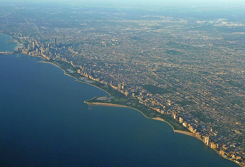 Before | 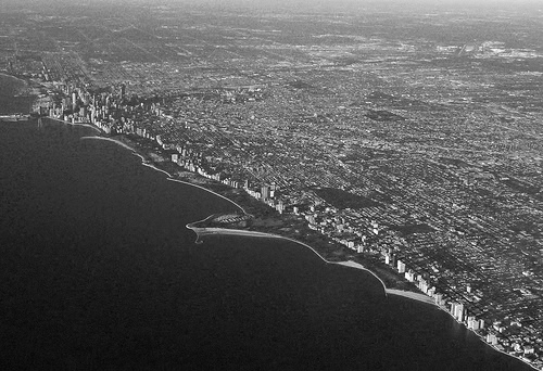 After |
Reclassification
SELECT ST_AsPNG(
   ST_Reclass(ST_Band(rast,1),1,'0-70:255, 71-189:100, 190-255:200', '8BUI',255)
   )
FROM po.chicago_pics
WHERE filename = 'Full_chicago_skyline.jpg';Before | 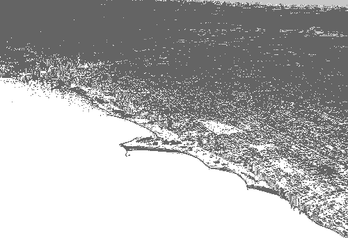 After |
Exercise: Resorting bands
There are good uses for this, but this is questionably not one of them.
SELECT ST_AsPNG(ST_Band(rast,'{3,2,1}'::integer[])) As png
  FROM po.chicago_pics
  WHERE filename='Full_chicago_skyline.jpg';
Before | 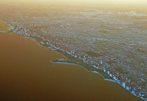 After |
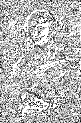
Roughness
You would do this with terrain data, but you could do it with pictures and create a charcoal drawing. Gives you relative measure of difference between max and min. Bears a striking resemblance to what you get when applying the ST_Range4MA mapalgebra callback function.
SELECT ST_AsPNG( ST_Roughness(rast,1, NULL::raster, '8BUI'::text) )
FROM chicago_pics
WHERE filename ILIKE 'Mona%';
Before | 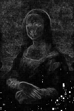 After |
Hillshade
Designed for elevation data (gives hypothetical illumination), but go ahead and apply to your pictures and create a stone impression.
SELECT ST_AsPNG( ST_HillShade(rast,1, NULL::raster, '8BUI'::text, 90) ) FROM chicago_pics WHERE filename ILIKE 'Mona%';SELECT ST_AsPNG( ST_HillShade(rast,1, NULL::raster, '8BUI'::text, 315,30,150) ) FROM chicago_pics WHERE filename ILIKE 'Mona%';
 Default (315 azimuth, 45 altitude, 255 max bright) | 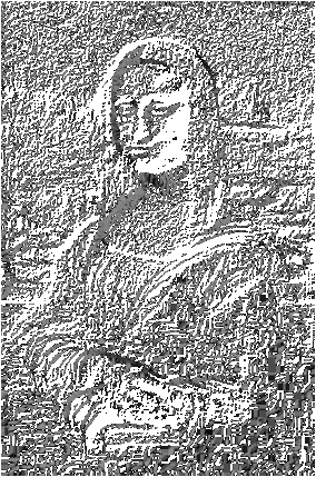 315, 30, 150 |
Aspect
Againt designed for elevation data, Returns the aspect (in degrees by default) of an elevation raster band.
SELECT ST_AsPNG( ST_Aspect(rast,1, NULL::raster, '8BUI'::text) )
FROM chicago_pics
WHERE filename ILIKE 'Mona%';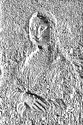 |
Map Algebra with ST_MapAlgebra
Operations done on a set of pixels (a neighborhood) where the value returned by the operation becomes the new value for the center pixel. The simplest operation works on a single cell (a 0-neighborhood).
In PostGIS the operation is expressed either as a PostgreSQL algebraic expression, or a Postgres callback function that takes an n-dimensional matrix of pixel values.
PostGIS has several built-in mapalgebra call-backs, but you can build your own. PostGIS packaged ones all have 4MA in them: 4MA means for Map Algebra
(ST_Min4MA, ST_Max4MA, ST_Mean4MA, ST_Range4MA (very similar to ST_Roughness), ST_InvDistWeight4MA, ST_Sum4MA)).
Default neighborhood is 0 distance from pixel in x direction, and 0 distance in y direction.
Map Algebra: Single-band
SELECT ST_AsPNG( ST_MapAlgebra(
    ARRAY[ROW(rast, 1)]::rastbandarg[],
    'ST_Min4MA(double precision[], int[], text[])'::regprocedure,
    '8BUI'::text, 'INTERSECTION'::text,
    NULL::raster,  1,1) )
FROM chicago_pics
WHERE filename ILIKE 'Mona%';
Min |  Mean |  Max |
ST_AddBand, MapAlgebra - apply to all bands
SELECT ST_AsPNG(ST_AddBand(NULL::raster,
  array_agg(ST_MapAlgebra(
    ARRAY[ROW(rast, i)]::rastbandarg[],
    'ST_Min4MA(double precision[], int[], text[])'::regprocedure,
    '8BUI'::text, 'INTERSECTION'::text,
    NULL::raster,  1,1
	) ) ) )
FROM chicago_pics CROSS JOIN generate_series(1,3) As i
WHERE filename ILIKE 'Mona%';
Before |  Min |  Max |
Exercise: Clipping
SELECT ST_Clip(rast, ST_Buffer(ST_Centroid(rast::geometry),100))
  FROM chicago_pics
  WHERE filename='Full_chicago_skyline.jpg';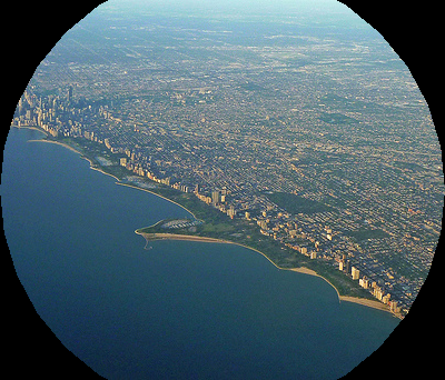
Setting band nodata values
SELECT ST_SetBandNoDataValue(
   ST_SetBandNoDataValue(
      ST_SetBandNoDataValue(
           ST_Clip(rast,
             ST_Buffer(ST_Centroid(rast::geometry),200) ),
              1,0),2,0),3,0)
  FROM chicago_pics
  WHERE filename='Full_chicago_skyline.jpg';
Resize, Shift, Union with SQL
SELECT ST_Union(
    ST_SetUpperLeft(
        ST_Resize(rast,i*0.3,i*0.3),i*150,i
        )
      )
  FROM chicago_pics CROSS JOIN generate_series(1,3) As i
  WHERE filename='Full_chicago_skyline.jpg';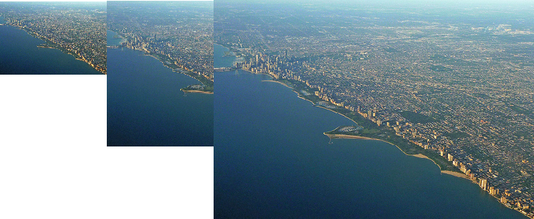
Now for something totally serious
People! Power of SQL is not for doodling
SQL should be used for REAL analysis and not to entertain your kids.
Exercise: Elevation at a point
SELECT ST_Value(rast,1,loc)
 FROM po.chicago_dem As d
  INNER JOIN
  ST_Transform(
    ST_SetSRID(ST_Point(-87.627,41.8819),4326),
        4267) As loc
    ON ST_Intersects(d.rast, loc);
181
Let's compare with Wikipedia's answer http://en.wikipedia.org/wiki/Chicago
Elevation [1](mean) 	594 ft (181 m)
Highest elevation
– near Blue Island 	672 ft (205 m)
Lowest elevation
– at Lake Michigan 	578 ft (176 m)
Exercise: Histogram of an area
Clip first to isolate region of interest
SELECT (h.hist).*
 FROM  ST_Transform(
    ST_Buffer(
       ST_Point(-87.627,41.8819)::geography,
       5000)::geometry,4267
        ) As loc,
  LATERAL
   (SELECT ST_Histogram(ST_Union(ST_Clip(rast,loc)),1,5) As hist
  FROM po.chicago_dem As d
    WHERE ST_Intersects(d.rast, loc) ) As h;
min | max | count | percent -----+-----+-------+---------------------- 166 | 171 | 5 | 0.00040983606557377 171 | 176 | 8 | 0.000655737704918033 176 | 181 | 7307 | 0.598934426229508 181 | 186 | 4414 | 0.361803278688525 186 | 191 | 466 | 0.0381967213114754 (5 rows)
Exercise: Quantiles of an area
Same exercise as histogram, but with Quants
SELECT (h.quant).*
 FROM  ST_Transform(
    ST_Buffer(
       ST_Point(-87.627,41.8819)::geography,
       5000)::geometry,4267
        ) As loc,
  LATERAL
     (SELECT
        ST_Quantile(ST_Union(ST_Clip(rast,loc)),1,
           '{0.1,0.5,0.75}'::float[]) As quant
        FROM po.chicago_dem As d
    WHERE ST_Intersects(d.rast, loc) ) As h;
quantile | value
----------+-------
0.1 | 176
0.5 | 178
0.75 | 181
(3 rows)
Transformation
Just like geometries we can transform raster data from one projection to another. Let's transform to web mercator to match our OSM chicago data
CREATE TABLE po.chicago_dem_wmerc AS
  SELECT rid, ST_Transform(rast, 900913) As rast
    FROM po.chicago_dem;
 SELECT AddRasterConstraints('po'::name,
  'chicago_dem_wmerc'::name, 'rast'::name);
Let's check meta data
After plain vanilla transformation
SELECT r_table_name, srid, scale_x::numeric(10,5),
  scale_y::numeric(10,5), blocksize_x As bx, blocksize_y As by,
   same_alignment As sa
  FROM raster_columns
  WHERE r_table_name LIKE 'chicago_dem%';
r_table_name | srid | scale_x | scale_y | bx | by | sa ------------------+--------+---------+----------+-----+-----+---- chicago_dem_wmerc | 900913 | | | 85 | 113 | f chicago_dem | 4267 | 0.00083 | -0.00083 | 100 | 100 | t
oh oh, new tiles have inconsistent alignment and scale
raster ST_Transform has many forms
In order to union and so forth, we need our tiles aligned
WITH ref As ( SELECT ST_Transform(rast,900913) As rast
      FROM po.chicago_dem LIMIT 1)
   SELECT d.rid, ST_Transform(d.rast,  ref.rast, 'Lanczos') As rast
    INTO po.chicago_dem_wmerc
   from ref CROSS JOIN po.chicago_dem As d;
We arbitrarily picked first transformed raster to align with
New raster meta data using aligned transform
After we repeat AddRasterConstraints and rerun our raster_columns query
   r_table_name    |  srid  |  scale_x  |  scale_y   | bx  | by  | sa
-------------------+--------+-----------+------------+-----+-----+----
 chicago_dem_wmerc | 900913 | 109.92805 | -109.92805 |  85 | 114 | t
 chicago_dem       |   4267 |   0.00083 |   -0.00083 | 100 | 100 | t
Index your rasters
CREATE INDEX idx_chicago_dem_wmerc_rast_gist
  ON po.chicago_dem_wmerc
  USING gist
  (st_convexhull(rast));
Colorize your dems with ST_ColorMap
DEMS are often not convertable to standard viewing formats like PNG, JPG, or GIF because their band types are often 16BUI, BSI and so forth rather than 8BUI.
With the beauty that is ST_ColorMap, you can change that.
INTERPOLATE, NEAREST, EXACT.
Named color map
There are: grayscale, pseudocolor, fire, bluered predefined in PostGIS. bluered goes from low of blue to pale white to red.
SELECT ST_ColorMap(ST_Union(rast,1),'bluered') As rast_4b
FROM po.chicago_dem_wmerc
 WHERE ST_DWithin(
    ST_Transform(ST_SetSRID(ST_Point(-87.627,41.8819),4326),900913),
        rast::geometry,5000);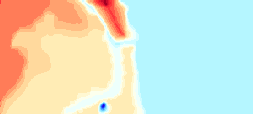
Custom color map
You can define mappings yourself
SELECT ST_ColorMap(ST_Union(rast,1),'100% 255 0 0
75% 200 0 0
50% 100 0 0
25% 50 0 0
10% 10 0 0
nv 0 0 0', 'INTERPOLATE') As rast_4b
FROM po.chicago_dem_wmerc
 WHERE ST_DWithin(
    ST_Transform(ST_SetSRID(ST_Point(-87.627,41.8819),4326),900913),
        rast::geometry,5000);
Custom color map
Fixed set of colors snap to nearest percentile
SELECT ST_ColorMap(ST_Union(rast,1),'100% 255 0 0
75% 200 0 0
50% 100 0 0
25% 50 0 0
10% 10 0 0
nv 0 0 0', 'NEAREST') As rast_4b
FROM po.chicago_dem_wmerc
 WHERE ST_DWithin(
    ST_Transform(ST_SetSRID(ST_Point(-87.627,41.8819),4326),900913),
        rast::geometry,5000);
Make 3D linestrings
WITH ref_D AS (SELECT name, way,
  ST_Transform(ST_SetSRID(ST_Point(-87.627,41.8819),4326),900913) As loc
   FROM po.planet_osm_roads
   ORDER BY ST_Transform(
    ST_SetSRID(
        ST_Point(-87.627,41.8819),4326),900913) <->  way LIMIT 5 ),
     ref AS (SELECT name, way FROM ref_d
       ORDER BY ST_Distance(way,loc) )
    SELECT ref.name,
        ST_AsText(
            ST_LineMerge(
                    ST_Collect(
                        ST_Translate(ST_Force3D((r.gv).geom), 0,0, (r.gv).val)
                  )
                )
            ) As wktgeom
        FROM
           ref , LATERAL (SELECT ST_Intersection(rast,way) As gv
              FROM po.chicago_dem_wmerc As d
                 WHERE ST_Intersects(d.rast, ref.way) ) As r
GROUP BY ref.name;3D linestring output
          name          |       wktgeom
------------------------+-------------------------------------------------------
 North State Street     | LINESTRING Z (-9754688.09 5143501.29 179,-9754687.4267
9796 5143457.79342028 179,-9754686.69 5143409.47 180,-9754684.13704138 5143347.8
6536781 180,-9754683.17 5143324.53 181) ...
 East Madison Street    | LINESTRING Z (-9754312.92 5143334.38 181,-9754328.32 5
143334.22 181,-9754407.28 5143333.33 181,-9754501.17 5143330.48 181,-9754587.69
5143329.8 181,-9754652.86 5143328.67 181,-9754666.75 5143327.67 181,-9754683.17
5143324.53 181)...
 State Street Subway    | MULTILINESTRING Z ((-9754692.86 5143480.52 179,-975469
2.09079665 5143457.79342028 179,-9754688.37017403 5143347.86536781 180,-9754680.
91 5143127.45 181),(-9754671.2 5143129.08 181,-9754677.91235681 5143347.86536781
 180,-9754681.28496038 5143457.79342028 179,-9754681.95 5143479.47 179)) ..
 East Washington Street | LINESTRING Z (-9754688.09 5143501.29 179,-9754591.31 5
143501.57 179,-9754538.75 5143500.92 179,-9754504.9 5143501.11 179,-9754410.36 5
143501.83 179,-9754316.66 5143502.34 179,-9754301.88 5143502.49 179,-9754289.33
5143502.58 179,-9754283.02 5143502.6 179) ...
(4 rows)
Exercise: Rasterizing a geometry
Basic ST_AsRaster
SELECT ST_AsPNG(ST_AsRaster(
  ST_Buffer(
        ST_GeomFromText('LINESTRING(50 50,150 150,150 65, 30 20)'),
            10,'join=bevel'),
            200,200,ARRAY['8BUI', '8BUI', '8BUI'],
    ARRAY[118,154,118], ARRAY[0,0,0]));
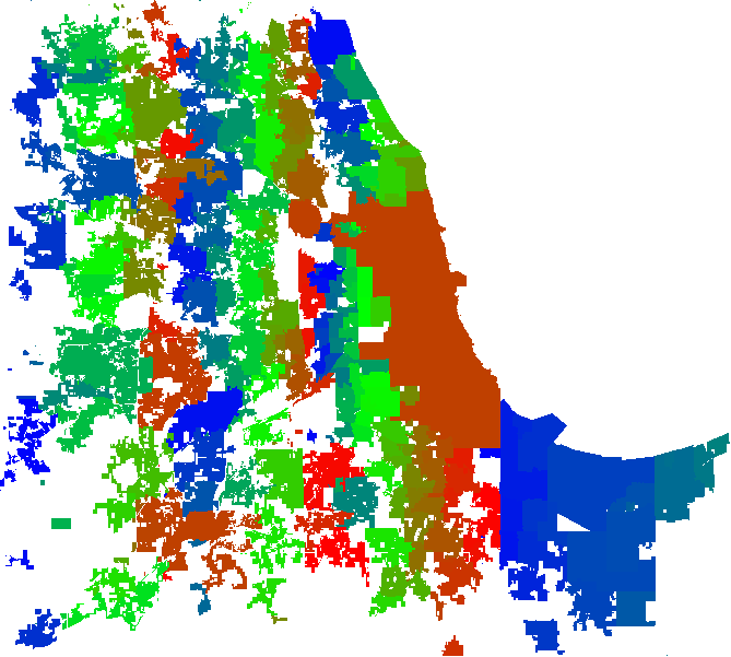
Exercise: Overlaying geometries on a grid + color mapping
ST_AsRaster variant 2
WITH cte AS (SELECT row_number() OVER() As rn, way As geom,
 ST_XMax(way) - ST_XMin(way) As width, ST_YMax(way) - ST_YMin(way) As height,
 ST_Extent(way) OVER() As full_ext
  FROM po.planet_osm_polygon
WHERE admin_level='8' ),
ref AS (SELECT ST_AsRaster(ST_SetSRID(full_ext, ST_SRID(geom)),
  ((ST_XMax(full_ext) - ST_XMin(full_ext))/
  (ST_YMax(full_ext) - ST_YMin(full_ext))*600)::integer,
    600,ARRAY['8BUI'],
    ARRAY[255], ARRAY[255]) AS rast FROM cte WHERE rn = 1 )
SELECT ST_AsPNG(ST_ColorMap(ST_Union(ST_AsRaster(geom, ref.rast,
    ARRAY['8BUI'],
   ARRAY[rn*2], ARRAY[255]) ), 'pseudocolor') )
FROM cte CROSS JOIN ref;
Raster output of overlay
Vectorizing portions of a raster
Most popular is ST_DumpAsPolygons which returns a set of geomval (composite consisting of a geometry named geom and a pixel value called val).
SELECT (g).val, ST_Union((g).geom) As geom
FROM
(SELECT ST_DumpAsPolygons(ST_Clip(rast,loc) ) As g
 FROM po.chicago_dem As d
  INNER JOIN
  ST_Transform(
    ST_Buffer(
        ST_SetSRID( ST_Point(-87.627,41.8819),4326)::geography,
        500 )::geometry,
        4267) As loc
    ON ST_Intersects(d.rast, loc) ) AS f
GROUP BY (g).val;
Topology: Geometries in seat-belts
Geometries are stand-alone selfish creatures.
They only look out for number one.
A plot of land overlaps another.
Does geometry care?
No. C'est la vie
People care. We've got boundaries. My land is not your land. Stay off my lawn.
Who can bring order to our world?
Topology can.
What is a topology?
Specifically: Network topology
Topology primitives: edges, nodes, and faces
Topology views the world as a neatly ordered network of faces, edges, and nodes. Via relationships of these primitive elements, we form recognizable things like parcels, roads, and political boundaries.
What is an edge?
An edge is a linestring that does not overlap other edges. It can only touch other edges at the end points.
What is a node?
Nodes are start and end points of edges or are isolated points that are not part of any edge.
What is a face?
A face is a polygon that gets generated when a set of edges form a closed ring.
In standard PostGIS topology, the polygon is never actually stored, but computed. Only the minimum bounding rectangle is stored.
Diagram of simple topology
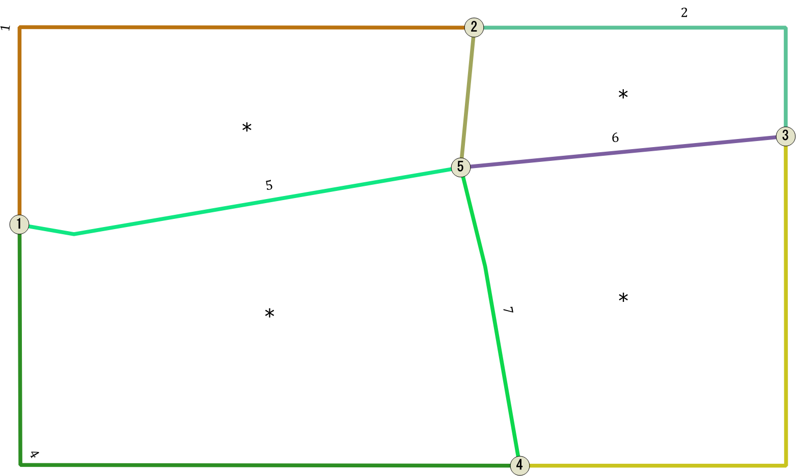
Edges are the numbered linestrings, nodes are the numbered round balls, and faces are the areas with *. The four faces together can be used to construct a topogeometry we can call colorado.
How does topology help us?
- Ensure correct boundaries
- When geometries are simplified shared edges still remain shared
- Editing
What is a topogeometry?
A topogeometry is like a geometry, except it has respect for its foundations. It understands it is not sitting by itself in outerspace. It understands it is made up of other elements which may be shared by other geometries. It understands its very definition is the cumulative definition of others.
It's nice to be a regular old geometry sometimes, and topogeometry has got a cast to make it so. topo::geometry or geometry(topo).
topogeometry is a set of relations
A topogeometry is composed of pointers to topology primitives or other topogeometries. It is defined via the relations
Let's build a topology of Chicago
With our OSM data
If you haven't already
CREATE EXTENSION postgis_topology;Create the topology
SELECT CreateTopology('topo_chicago',900913);You should now have a database schema called topo_chicago with several tables.
Tables in a topology
topo_chicago has a set of tables you'll find in all topology generated schemas
- edge_data and companion edge view: Holds all the line work that defines the topological network.
- node - defines all the points that connect the edges (only connecting points are considered) as well as isolated points (isonode) that stand alone.
- face - lists polygons formed by closed line work of edges. The polygon is not stored, only the minimum bounding box
- relation - lists the set of relationships to edges, nodes, faces, and other layers that define a topogoemetry.
Let's create a political boundaries table from scratch
CREATE TABLE
  po.chicago_boundaries(id serial primary key,  name text);
SELECT AddTopoGeometryColumn('topo_chicago', 'po',
 'chicago_boundaries', 'topo', 'POLYGON') As layer_id;
1
Let's populate our boundaries
INSERT INTO po.chicago_boundaries(name, topo)
WITH ref AS (SELECT way As ref
    FROM po.planet_osm_polygon
    WHERE admin_level = '8' AND name = 'Chicago')
SELECT name,  toTopoGeom(ST_Union(way), 'topo_chicago', 1)
    FROM (SELECT name, way FROM po.planet_osm_polygon
    WHERE admin_level = '8') AS b
    INNER JOIN ref
ON (ST_Intersects(b.way,ref.ref))
GROUP BY name;
Output topogeometry as geometry
SELECT name, topo::geometry As geom
 FROM po.chicago_boundaries;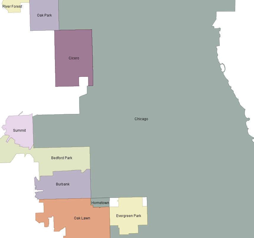
Simplify topo boundaries compared to simplify geometry boundaries
Topos are aware of their shared existence. Edges remain shared.
Geometries are self-centered. They don't care about their neighbors.
Chicago Geometry simplified
They overlap and are not respectful of each other.
SELECT name, ST_Simplify(topo::geometry,1000) As geom
 FROM po.chicago_boundaries;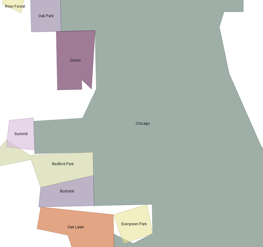
Chicago TopoGeometry simplified
Edges that were shared are still shared
SELECT name, ST_Simplify(topo,1000) As geom
 FROM po.chicago_boundaries;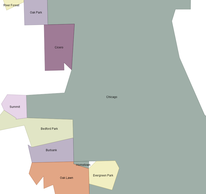
pgRouting: Navigating from one place to another
pgRouting is primarily used for building routing applications. E.g road directions, biking trail guide etc.
Install binaries
Refer to our quick start guide listed on this page: http://www.postgis.us/pgopen2014
Enable in your database and verify
CREATE EXTENSION pgrouting;
SELECT * FROM pgr_version();
version |  tag   | build |  hash   | branch | boost
---------+--------+-------+---------+--------+--------
 2.0.0   | v2.0.0 | 3     | fbbaa2a | master | 1.54.0
Popular tools for making OSM data routable
- osm2pgrouting osm2pgrouting - not tested on windows.
- osm2po - http://osm2po.de works on any OS with a java VM. Other neat feature is it comes with its own mini-webserver that reads the .pbf file directly.
We'll demonstrate osm2po since it's more cross-platform
Prepping data for routing with osm2po
- Extract osm2po in a folder: we used the 4.8.8 version
- Make a copy of the demo.bat or demo.sh and replace with your own path to pbf
- If java is not in your path, you may need to define a path variable at top
Generating sql script for routing chicago
Your shell-script line should look something like
java -Xmx512m -jar osm2po-core-4.8.8-signed.jar prefix=hh tileSize=x chicago_illinois.osm.pbfYou should now have a folder called hh in your osm2po folder, and should have an sql file hh_2po_4pgr.sql
Load this up into your database with psql. Note that osm2po loads data in wgs 84 long lat geometry (4326) so tolerance units for all pgrouting will be in degrees.
Recreate vertices from source and target
Osm2Po doesn't create a vertices table, but we can create one from the table it creates. This table is needed by some pgrouting functions
SELECT pgr_createVerticesTable('hh_2po_4pgr', 'geom_way', 'source', 'target')NOTICE: PROCESSING:
NOTICE: pgr_createVerticesTable('hh_2po_4pgr','geom_way','source','target','true')
NOTICE: Performing checks, pelase wait .....
NOTICE: Populating public.hh_2po_4pgr_vertices_pgr, please wait...
NOTICE: -----> VERTICES TABLE CREATED WITH 338965 VERTICES
NOTICE: FOR 489747 EDGES
NOTICE: Edges with NULL geometry,source or target: 0
NOTICE: Edges processed: 489747
NOTICE: Vertices table for table public.hh_2po_4pgr is: public.hh_2po_4pgr_vertices_pgr
NOTICE: ----------------------------------------------
Total query runtime: 42975 ms.
Analyzing your routes
pgr_analyzeGraph looks for dead ends and other anomalies and populates fields in hh_2po_4pgr_vertices_pgr. Tolerance are in units of your spatial ref sys. Takes a while
SELECT pgr_analyzeGraph('hh_2po_4pgr', 0.000001,'geom_way',
'id', 'source', 'target','true');OK120,322ms
Using osm2po routing table
Create view with key columns we need
CREATE OR REPLACE VIEW vw_routing
AS
SELECT id, osm_id, osm_name, osm_meta, osm_source_id, osm_target_id,
       clazz, flags, source, target, km, kmh, cost,
	   cost as length, reverse_cost, x1,
       y1, x2, y2, geom_way As the_geom
  FROM hh_2po_4pgr;
pgRouting is about going from one node to another along a path not really about location
So we really can't go from arbitrary point to point, have to go from node to node. So we found a node using osm2po mini webservice: http://localhost:8888/Osm2poService
pgr_astar
Shortest Path A-Star function that takes as input:
- SQL statement that defines your network or portion of network you want to inspect
- node id of start
- node id of end
- directed: defaults to true (if your graph has direction)
- has_rcost: If your edges have costs in different direction. reverse_cost must be provided if this is true
Directed route with astar
Output is order of travel: seq, id1: node id, id2 edge id
SELECT *
  FROM pgr_astar('SELECT id, source, target, cost,
  x1,y1,x2,y2, reverse_cost FROM vw_routing',
               159944, 142934, true, true) As r;
seq | id1 | id2 | cost -----+--------+--------+-------------- 0 | 159944 | 236443 | 0.0020273041 1 | 334003 | 482441 | 0.0027647596 2 | 334007 | 482442 | 0.0010009945 3 | 334006 | 155460 | 0.0025687038 4 | 142934 | -1 | 0
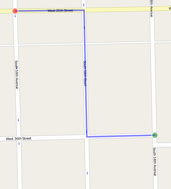
Directed route with astar joined with road
One-ways are considered
SELECT r.seq, r.id1 As node,
	s.id As edge, s.osm_name, s.cost, s.km, s.kmh
  FROM pgr_astar('SELECT id, source, target, cost,
  x1,y1,x2,y2, reverse_cost FROM vw_routing',
               159944, 142934, true, true) As r INNER JOIN
        vw_routing AS s ON r.id2 =  s.id
	ORDER BY r.seq;
seq | node | edge | osm_name | cost | km | kmh ----+--------+--------+------------------+--------------+-------------+----- 0 | 159944 | 236443 | West 36th Street | 0.0020273041 | 0.10136521 | 50 1 | 334003 | 482441 | South 58th Court | 0.0027647596 | 0.13823798 | 50 2 | 334007 | 482442 | South 58th Court | 0.0010009945 | 0.050049722 | 50 3 | 334006 | 155460 | West 35th Street | 0.0025687038 | 0.102748156 | 40
Undirected route with astar joined with road
One-ways are ignored
SELECT r.seq, r.id1 As node,
	s.id As edge, s.osm_name, s.cost, s.km, s.kmh
  FROM pgr_astar('SELECT id, source, target, cost,
  x1,y1,x2,y2, reverse_cost FROM vw_routing',
               159944, 142934, false, false) As r INNER JOIN
        vw_routing AS s ON r.id2 =  s.id
	ORDER BY r.seq;
seq | node | edge | osm_name | cost | km | kmh -----+--------+--------+-------------------+--------------+-------------+----- 0 | 159944 | 236443 | West 36th Street | 0.0020273041 | 0.10136521 | 50 1 | 334003 | 236444 | West 36th Street | 0.0020233293 | 0.101166464 | 50 2 | 333993 | 482429 | South 59th Avenue | 0.0027747066 | 0.13873532 | 50 3 | 333996 | 482428 | South 59th Avenue | 0.0010170189 | 0.050850946 | 50
Links of Interest
THE END
Thank you. Buy our books http://www.postgis.us
- The Paragon Logo is copyright Paragon Corporation and may be resized, made transparent and so forth. It should only be used to refer to Paragon Corporation.
- Many of the raster images used in this presentation were downloaded from Wikipedia. The ones of Mona Lisa are resized versions of Mona Lisa which is under a public domain license.
- The aerial clip is a portion of Massachusetts aerial data loaded in PostGIS raster format from MassGIS 2008/2009 aerial data. This particular clip is borrowed from the PostGIS documentation which is under a Creative Commons 3.0 Share Alike
- Images of Chicago: were taken from this http://en.wikipedia.org/wiki/Chicago page and under the respective licenses of the photographers.
- Slide were made using RevealJS which is MIT Licensed